Tonpilz TVR Analyzer

This tool estimates the Transmitting Voltage Response (TVR) of a tonpilz-type underwater transducer using a 1D lumped Mason equivalent-circuit model. All calculations run in the browser with no server or external dependency.

The model solves a two-mass / one-spring system in the frequency domain: the tail mass (body + bolt + half PZT stack) and the head mass (piston + optional matching layer + half PZT stack) are coupled through an effective spring that combines PZT stack stiffness, bolt stiffness, piston compliance, and body compliance in series/parallel. Radiation into the surrounding medium is modelled by the exact baffled-piston radiation impedance (Beranek, using Bessel and Struve functions).

2. Interface

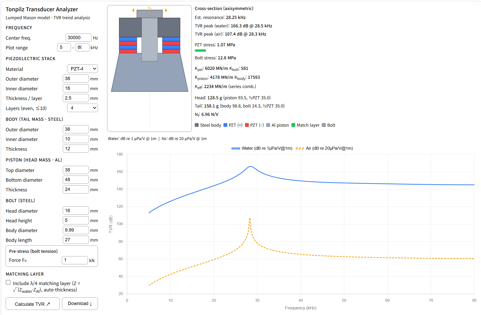
Fig. 1 — Tool interface. Left panel: inputs. Right panel top: cross-section diagram. Right panel bottom: TVR graph.

Buttons

Validation checks

The tool performs basic geometric consistency checks before calculating (e.g. bolt diameter vs. body inner diameter, bolt length vs. stack + body height) and displays an error message if any constraint is violated. The center frequency is restricted to 100 Hz – 100 kHz.

3. Physical Model

3.1 Effective stiffness

Four spring elements are combined. The PZT stack (short-circuit stiffness) and the pre-stressed bolt act in parallel; that sub-assembly, the piston frustum, and the body cylinder then act in series:

where K_pzt = A_pzt / (s33_E × h_stack), K_bolt = E_steel × A_bolt / L_bolt, K_piston = π × E_Al × r_top × r_bot / h_piston, K_body = E_steel × A_body / h_body.

Pre-stress modifies the PZT stiffness through a stress-stiffening factor (empirical, ~8 % per unit normalised stress).

3.2 Effective masses

The PZT stack mass is split equally between head and tail. Head mass = piston + ½ PZT + matching layer (if present). Tail mass = body + bolt assembly + ½ PZT.

3.3 Radiation impedance

The radiation face is taken as the bottom face of the piston (or matching layer if present). The baffled circular-piston radiation impedance is computed analytically:

using the exact series expansions for R₁ (Bessel J₁) and X₁ (Struve H₁). This is exact for ka up to any value, not just the low-frequency approximation.

3.4 Matching layer

When selected, a quarter-wavelength layer is added at the radiation face. Its acoustic impedance is set to the geometric mean of water and aluminium: Z_m = √(Z_water × Z_Al). Its thickness is h = c_m / (4 × f_center), computed automatically. The layer is modelled as a transmission-line transformer applied to the radiation impedance before entering the mechanical network.

3.5 Force factor and TVR

The force factor is N_f = d33 × A_pzt / (s33_E × t_layer), consistent with parallel electrical connection of N layers. The head-mass velocity v_h is obtained by solving the 2-port Mason network, and the far-field pressure at 1 m is p(1m) = ρ c k a² / 2 × |v_h|.

4. Validity and Limitations

The model gives reliable trend predictions when:

The piston bottom diameter is close to the PZT outer diameter (ratio ≤ ~1.5). In this regime the piston moves essentially as a rigid body and the 1D spring-mass assumption holds.
The frequency of interest is near and below the fundamental longitudinal resonance (roughly within one octave).
A single dominant resonance governs the TVR (typical for well-designed tonpilz transducers with a large tail-to-head mass ratio).
You need fast parametric sweeps to compare design variants — the tool responds instantly and gives consistent relative trends.

The model is NOT reliable when:

The piston is significantly wider than the PZT stack. When the piston outer diameter greatly exceeds the PZT outer diameter, the piston no longer moves as a rigid body. Flexural (bending) modes in the piston dominate the dynamic compliance, making the effective stiffness orders of magnitude lower than predicted by the 1D model. The computed resonance frequency will then be far too high and the TVR curve shape will be qualitatively wrong.
Higher-order or flexural modes are important. Multiple resonance peaks in the operating band, or transducers designed to exploit piston flexure, cannot be captured in a 1D framework.
Frequencies well above resonance (beyond ~2× the fundamental). The lumped assumption (all dimensions ≪ wavelength in each part) breaks down.
Absolute TVR accuracy is required. Even in the valid regime (see below), the model systematically over-predicts TVR amplitude. It should be used for relative comparisons and trend analysis only.

5. Comparison with COMSOL

5.1 Case A — large tonpilz (PZT OD ≈ piston OD)

The following geometry is taken from the COMSOL Application Library (Tonpilz Transducer example) and represents a well-proportioned design where the piston outer diameter is close to the PZT outer diameter.

Input parameters — Case A (COMSOL Application Library v.5.4 example)
Component	Parameter	Value
PZT-4 stack	Outer / inner diameter	38 / 16 mm
Thickness per layer	2.5 mm
Number of layers	4

Body (steel)	Outer / inner diameter	38 / 10 mm
Thickness	12 mm

Piston (Al)	Top / bottom diameter	38 / 48 mm
Thickness	24 mm

Bolt (steel)	Head diameter / height	16 / 5 mm
Body diameter / length	9.99 / 27 mm
Pre-stress	1 kN

Matching layer		None

Results comparison — Case A
	COMSOL (FEM)	This tool (lumped)	Difference
Resonance frequency	~28 kHz	~28 kHz	≈ 0 %
TVR peak (water)	~152 dB re 1 μPa/V @ 1m	~166 dB re 1 μPa/V @ 1m	+14 dB

Interpretation: The resonance frequency is well predicted. The TVR amplitude is over-predicted by approximately 14 dB. This systematic offset arises because the 1D model assumes a perfectly rigid piston radiating as a uniform piston, whereas in reality the piston has finite compliance and the velocity distribution across its face is non-uniform. The tool is therefore suitable for comparing relative TVR levels between design variants (e.g. the effect of changing PZT stack height or head mass), but not for predicting the absolute dB level.

5.2 Case B — small tonpilz (piston OD ≫ PZT OD)

A second case uses a smaller geometry where the piston bottom diameter (25 mm) is more than twice the PZT outer diameter (12 mm).

Input parameters — Case B
Component	Parameter	Value
PZT-4 stack	Outer / inner diameter	12 / 8 mm
Thickness / layers	2 mm × 4

Body (steel)	OD / ID / thickness	16 / 4 / 10 mm
Piston (Al)	top ⌀ / bottom ⌀ / thickness	20 / 25 / 7 mm
Bolt	head ⌀×h / body ⌀×L	8×2 mm / 3.99×20 mm

Results comparison — Case B
	COMSOL (FEM)	This tool (lumped)
Resonance frequency	~8 kHz (primary), ~35 kHz (secondary)	~44 kHz
TVR curve shape	Two distinct peaks; flat plateau between	Single monotone rise to one peak

This case is outside the valid range of the 1D model. The piston-to-PZT diameter ratio exceeds 2×, so piston flexure dominates. The effective stiffness seen by the piston is ~30× lower than the 1D model predicts, shifting the true resonance from ~44 kHz down to ~8 kHz. The secondary peak at ~35 kHz is a 2D flexural mode of the piston that cannot be captured in any 1D framework. For geometries of this type, a 2D axisymmetric FEM (e.g. COMSOL, or a custom Python/SfePy implementation) is required.

6. Summary

Quantity	Reliability	Notes
Resonance frequency (valid regime)	Good	Typically within 5–10 % if piston OD ≤ 1.5 × PZT OD
TVR curve shape (valid regime)	Good (qualitative)	Peak location and roll-off trend are correctly reproduced
TVR absolute level	Poor	Systematically over-predicted; typical offset ~10–15 dB
Resonance frequency (invalid regime)	Poor	Can be 2–5× too high when piston flexure dominates
Multiple resonance peaks	Not supported	Model produces only one mechanical resonance

Material constants used in the model: PZT-4 s₃₃^E = 15.5×10⁻¹² m²/N, d₃₃ = 289×10⁻¹² C/N, ρ = 7500 kg/m³, Q_m = 500; Steel E = 205 GPa, ρ = 7850 kg/m³; Aluminium E = 70 GPa, ρ = 2700 kg/m³. These are standard handbook values and differ slightly from the COMSOL material library; the difference has a minor effect on resonance frequency (≲ 2 %) and does not explain the TVR amplitude discrepancy.

1. Overview